Open In Colab

About

This notebook is a demonstration of some Data Visulaization capabilities of Google Colab.

Introduction to Matplotlib and Line Plots

Exploring Datasets with pandas

pandas is an essential data analysis toolkit for Python. From their website:

pandas is a Python package providing fast, flexible, and expressive data structures designed to make working with “relational” or “labeled” data both easy and intuitive. It aims to be the fundamental high-level building block for doing practical, real world data analysis in Python.

The course heavily relies on pandas for data wrangling, analysis, and visualization. We encourage you to spend some time and familizare yourself with the pandas API Reference:http://pandas.pydata.org/pandas-docs/stable/api.html.

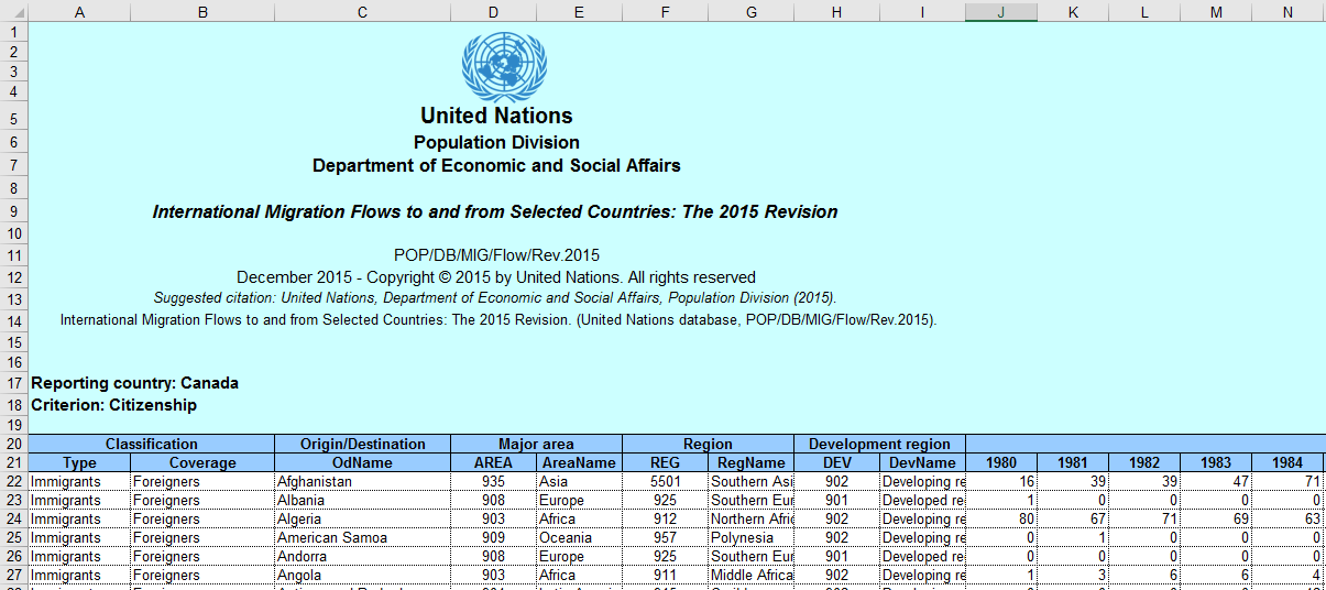
The Dataset: Immigration to Canada from 1980 to 2013

Dataset Source: International migration flows to and from selected countries - The 2015 revision.

The dataset contains annual data on the flows of international immigrants as recorded by the countries of destination. The data presents both inflows and outflows according to the place of birth, citizenship or place of previous / next residence both for foreigners and nationals. The current version presents data pertaining to 45 countries.

In this lab, we will focus on the Canadian immigration data.

`

For sake of simplicity, Canada's immigration data has been extracted and uploaded to one of IBM servers. You can fetch the data from here.


pandas Basics

The first thing we'll do is import two key data analysis modules: pandas and Numpy.

import numpy as np  # useful for many scientific computing in Python
import pandas as pd # primary data structure library

Let's download and import our primary Canadian Immigration dataset using pandas read_excel() method. Normally, before we can do that, we would need to download a module which pandas requires to read in excel files. This module is xlrd. For your convenience, we have pre-installed this module, so you would not have to worry about that. Otherwise, you would need to run the following line of code to install the xlrd module:

!conda install -c anaconda xlrd --yes

Now we are ready to read in our data.

df_can = pd.read_excel('https://s3-api.us-geo.objectstorage.softlayer.net/cf-courses-data/CognitiveClass/DV0101EN/labs/Data_Files/Canada.xlsx',
                       sheet_name='Canada by Citizenship',
                       skiprows=range(20),
                       skipfooter=2)

print ('Data read into a pandas dataframe!')
Data read into a pandas dataframe!

Let's view the top 5 rows of the dataset using the head() function.

df_can.head()
# tip: You can specify the number of rows you'd like to see as follows: df_can.head(10) 
Type Coverage OdName AREA AreaName REG RegName DEV DevName 1980 1981 1982 1983 1984 1985 1986 1987 1988 1989 1990 1991 1992 1993 1994 1995 1996 1997 1998 1999 2000 2001 2002 2003 2004 2005 2006 2007 2008 2009 2010 2011 2012 2013
0 Immigrants Foreigners Afghanistan 935 Asia 5501 Southern Asia 902 Developing regions 16 39 39 47 71 340 496 741 828 1076 1028 1378 1170 713 858 1537 2212 2555 1999 2395 3326 4067 3697 3479 2978 3436 3009 2652 2111 1746 1758 2203 2635 2004
1 Immigrants Foreigners Albania 908 Europe 925 Southern Europe 901 Developed regions 1 0 0 0 0 0 1 2 2 3 3 21 56 96 71 63 113 307 574 1264 1816 1602 1021 853 1450 1223 856 702 560 716 561 539 620 603
2 Immigrants Foreigners Algeria 903 Africa 912 Northern Africa 902 Developing regions 80 67 71 69 63 44 69 132 242 434 491 872 795 717 595 1106 2054 1842 2292 2389 2867 3418 3406 3072 3616 3626 4807 3623 4005 5393 4752 4325 3774 4331
3 Immigrants Foreigners American Samoa 909 Oceania 957 Polynesia 902 Developing regions 0 1 0 0 0 0 0 1 0 1 2 0 0 0 0 0 0 0 0 0 0 0 0 0 0 0 1 0 0 0 0 0 0 0
4 Immigrants Foreigners Andorra 908 Europe 925 Southern Europe 901 Developed regions 0 0 0 0 0 0 2 0 0 0 3 0 1 0 0 0 0 0 2 0 0 1 0 2 0 0 1 1 0 0 0 0 1 1

We can also veiw the bottom 5 rows of the dataset using the tail() function.

df_can.tail()
Type Coverage OdName AREA AreaName REG RegName DEV DevName 1980 1981 1982 1983 1984 1985 1986 1987 1988 1989 1990 1991 1992 1993 1994 1995 1996 1997 1998 1999 2000 2001 2002 2003 2004 2005 2006 2007 2008 2009 2010 2011 2012 2013
190 Immigrants Foreigners Viet Nam 935 Asia 920 South-Eastern Asia 902 Developing regions 1191 1829 2162 3404 7583 5907 2741 1406 1411 3004 3801 5870 5416 6547 5105 3723 2462 1752 1631 1419 1803 2117 2291 1713 1816 1852 3153 2574 1784 2171 1942 1723 1731 2112
191 Immigrants Foreigners Western Sahara 903 Africa 912 Northern Africa 902 Developing regions 0 0 0 0 0 0 0 0 0 0 0 1 0 0 0 0 0 0 0 0 0 0 0 0 0 0 1 0 0 0 0 0 0 0
192 Immigrants Foreigners Yemen 935 Asia 922 Western Asia 902 Developing regions 1 2 1 6 0 18 7 12 7 18 4 18 41 41 39 73 144 121 141 134 122 181 171 113 124 161 140 122 133 128 211 160 174 217
193 Immigrants Foreigners Zambia 903 Africa 910 Eastern Africa 902 Developing regions 11 17 11 7 16 9 15 23 44 68 77 69 73 46 51 41 34 72 34 51 39 78 50 46 56 91 77 71 64 60 102 69 46 59
194 Immigrants Foreigners Zimbabwe 903 Africa 910 Eastern Africa 902 Developing regions 72 114 102 44 32 29 43 68 99 187 129 94 61 72 78 58 39 44 43 49 98 110 191 669 1450 615 454 663 611 508 494 434 437 407

When analyzing a dataset, it's always a good idea to start by getting basic information about your dataframe. We can do this by using the info() method.

df_can.info()
<class 'pandas.core.frame.DataFrame'>
RangeIndex: 195 entries, 0 to 194
Data columns (total 43 columns):
 #   Column    Non-Null Count  Dtype 
---  ------    --------------  ----- 
 0   Type      195 non-null    object
 1   Coverage  195 non-null    object
 2   OdName    195 non-null    object
 3   AREA      195 non-null    int64 
 4   AreaName  195 non-null    object
 5   REG       195 non-null    int64 
 6   RegName   195 non-null    object
 7   DEV       195 non-null    int64 
 8   DevName   195 non-null    object
 9   1980      195 non-null    int64 
 10  1981      195 non-null    int64 
 11  1982      195 non-null    int64 
 12  1983      195 non-null    int64 
 13  1984      195 non-null    int64 
 14  1985      195 non-null    int64 
 15  1986      195 non-null    int64 
 16  1987      195 non-null    int64 
 17  1988      195 non-null    int64 
 18  1989      195 non-null    int64 
 19  1990      195 non-null    int64 
 20  1991      195 non-null    int64 
 21  1992      195 non-null    int64 
 22  1993      195 non-null    int64 
 23  1994      195 non-null    int64 
 24  1995      195 non-null    int64 
 25  1996      195 non-null    int64 
 26  1997      195 non-null    int64 
 27  1998      195 non-null    int64 
 28  1999      195 non-null    int64 
 29  2000      195 non-null    int64 
 30  2001      195 non-null    int64 
 31  2002      195 non-null    int64 
 32  2003      195 non-null    int64 
 33  2004      195 non-null    int64 
 34  2005      195 non-null    int64 
 35  2006      195 non-null    int64 
 36  2007      195 non-null    int64 
 37  2008      195 non-null    int64 
 38  2009      195 non-null    int64 
 39  2010      195 non-null    int64 
 40  2011      195 non-null    int64 
 41  2012      195 non-null    int64 
 42  2013      195 non-null    int64 
dtypes: int64(37), object(6)
memory usage: 65.6+ KB

To get the list of column headers we can call upon the dataframe's .columns parameter.

df_can.columns.values 
array(['Type', 'Coverage', 'OdName', 'AREA', 'AreaName', 'REG', 'RegName',
       'DEV', 'DevName', 1980, 1981, 1982, 1983, 1984, 1985, 1986, 1987,
       1988, 1989, 1990, 1991, 1992, 1993, 1994, 1995, 1996, 1997, 1998,
       1999, 2000, 2001, 2002, 2003, 2004, 2005, 2006, 2007, 2008, 2009,
       2010, 2011, 2012, 2013], dtype=object)

Similarly, to get the list of indicies we use the .index parameter.

df_can.index.values
array([  0,   1,   2,   3,   4,   5,   6,   7,   8,   9,  10,  11,  12,
        13,  14,  15,  16,  17,  18,  19,  20,  21,  22,  23,  24,  25,
        26,  27,  28,  29,  30,  31,  32,  33,  34,  35,  36,  37,  38,
        39,  40,  41,  42,  43,  44,  45,  46,  47,  48,  49,  50,  51,
        52,  53,  54,  55,  56,  57,  58,  59,  60,  61,  62,  63,  64,
        65,  66,  67,  68,  69,  70,  71,  72,  73,  74,  75,  76,  77,
        78,  79,  80,  81,  82,  83,  84,  85,  86,  87,  88,  89,  90,
        91,  92,  93,  94,  95,  96,  97,  98,  99, 100, 101, 102, 103,
       104, 105, 106, 107, 108, 109, 110, 111, 112, 113, 114, 115, 116,
       117, 118, 119, 120, 121, 122, 123, 124, 125, 126, 127, 128, 129,
       130, 131, 132, 133, 134, 135, 136, 137, 138, 139, 140, 141, 142,
       143, 144, 145, 146, 147, 148, 149, 150, 151, 152, 153, 154, 155,
       156, 157, 158, 159, 160, 161, 162, 163, 164, 165, 166, 167, 168,
       169, 170, 171, 172, 173, 174, 175, 176, 177, 178, 179, 180, 181,
       182, 183, 184, 185, 186, 187, 188, 189, 190, 191, 192, 193, 194])

Note: The default type of index and columns is NOT list.

print(type(df_can.columns))
print(type(df_can.index))
<class 'pandas.core.indexes.base.Index'>
<class 'pandas.core.indexes.range.RangeIndex'>

To get the index and columns as lists, we can use the tolist() method.

df_can.columns.tolist()
df_can.index.tolist()

print (type(df_can.columns.tolist()))
print (type(df_can.index.tolist()))
<class 'list'>
<class 'list'>

To view the dimensions of the dataframe, we use the .shape parameter.

# size of dataframe (rows, columns)
df_can.shape   
(195, 43)

Note: The main types stored in pandas objects are float, int, bool, datetime64[ns] and datetime64[ns, tz] (in >= 0.17.0), timedelta[ns], category (in >= 0.15.0), and object (string). In addition these dtypes have item sizes, e.g. int64 and int32.

Let's clean the data set to remove a few unnecessary columns. We can use pandas drop() method as follows:

# in pandas axis=0 represents rows (default) and axis=1 represents columns.
df_can.drop(['AREA','REG','DEV','Type','Coverage'], axis=1, inplace=True)
df_can.head(2)
OdName AreaName RegName DevName 1980 1981 1982 1983 1984 1985 1986 1987 1988 1989 1990 1991 1992 1993 1994 1995 1996 1997 1998 1999 2000 2001 2002 2003 2004 2005 2006 2007 2008 2009 2010 2011 2012 2013
0 Afghanistan Asia Southern Asia Developing regions 16 39 39 47 71 340 496 741 828 1076 1028 1378 1170 713 858 1537 2212 2555 1999 2395 3326 4067 3697 3479 2978 3436 3009 2652 2111 1746 1758 2203 2635 2004
1 Albania Europe Southern Europe Developed regions 1 0 0 0 0 0 1 2 2 3 3 21 56 96 71 63 113 307 574 1264 1816 1602 1021 853 1450 1223 856 702 560 716 561 539 620 603

Let's rename the columns so that they make sense. We can use rename() method by passing in a dictionary of old and new names as follows:

df_can.rename(columns={'OdName':'Country', 'AreaName':'Continent', 'RegName':'Region'}, inplace=True)
df_can.columns
Index([  'Country', 'Continent',    'Region',   'DevName',        1980,
              1981,        1982,        1983,        1984,        1985,
              1986,        1987,        1988,        1989,        1990,
              1991,        1992,        1993,        1994,        1995,
              1996,        1997,        1998,        1999,        2000,
              2001,        2002,        2003,        2004,        2005,
              2006,        2007,        2008,        2009,        2010,
              2011,        2012,        2013],
      dtype='object')

We will also add a 'Total' column that sums up the total immigrants by country over the entire period 1980 - 2013, as follows:

df_can['Total'] = df_can.sum(axis=1)

We can check to see how many null objects we have in the dataset as follows:

df_can.isnull().sum()
Country      0
Continent    0
Region       0
DevName      0
1980         0
1981         0
1982         0
1983         0
1984         0
1985         0
1986         0
1987         0
1988         0
1989         0
1990         0
1991         0
1992         0
1993         0
1994         0
1995         0
1996         0
1997         0
1998         0
1999         0
2000         0
2001         0
2002         0
2003         0
2004         0
2005         0
2006         0
2007         0
2008         0
2009         0
2010         0
2011         0
2012         0
2013         0
Total        0
dtype: int64

Finally, let's view a quick summary of each column in our dataframe using the describe() method.

df_can.describe()
1980 1981 1982 1983 1984 1985 1986 1987 1988 1989 1990 1991 1992 1993 1994 1995 1996 1997 1998 1999 2000 2001 2002 2003 2004 2005 2006 2007 2008 2009 2010 2011 2012 2013 Total
count 195.000000 195.000000 195.000000 195.000000 195.000000 195.000000 195.000000 195.000000 195.000000 195.000000 195.000000 195.000000 195.000000 195.000000 195.000000 195.000000 195.000000 195.000000 195.000000 195.000000 195.000000 195.000000 195.000000 195.000000 195.000000 195.000000 195.000000 195.000000 195.000000 195.000000 195.000000 195.000000 195.000000 195.000000 195.000000
mean 508.394872 566.989744 534.723077 387.435897 376.497436 358.861538 441.271795 691.133333 714.389744 843.241026 964.379487 1064.148718 1136.856410 1138.712821 993.153846 962.625641 1026.076923 989.153846 824.241026 922.143590 1111.343590 1244.323077 1144.158974 1114.343590 1190.169231 1320.292308 1266.958974 1191.820513 1246.394872 1275.733333 1420.287179 1262.533333 1313.958974 1320.702564 32867.451282
std 1949.588546 2152.643752 1866.997511 1204.333597 1198.246371 1079.309600 1225.576630 2109.205607 2443.606788 2555.048874 3158.730195 2952.093731 3330.083742 3495.220063 3613.336444 3091.492343 3321.045004 3070.761447 2385.943695 2887.632585 3664.042361 3961.621410 3660.579836 3623.509519 3710.505369 4425.957828 3926.717747 3443.542409 3694.573544 3829.630424 4462.946328 4030.084313 4247.555161 4237.951988 91785.498686
min 0.000000 0.000000 0.000000 0.000000 0.000000 0.000000 0.000000 0.000000 0.000000 0.000000 0.000000 0.000000 0.000000 0.000000 0.000000 0.000000 0.000000 0.000000 0.000000 0.000000 0.000000 0.000000 0.000000 0.000000 0.000000 0.000000 0.000000 0.000000 0.000000 0.000000 0.000000 0.000000 0.000000 0.000000 1.000000
25% 0.000000 0.000000 0.000000 0.000000 0.000000 0.000000 0.500000 0.500000 1.000000 1.000000 2.000000 3.000000 6.500000 11.500000 9.500000 10.500000 14.500000 19.500000 15.000000 16.000000 16.000000 22.000000 18.500000 21.500000 19.000000 28.500000 25.000000 31.000000 31.000000 36.000000 40.500000 37.500000 42.500000 45.000000 952.000000
50% 13.000000 10.000000 11.000000 12.000000 13.000000 17.000000 18.000000 26.000000 34.000000 44.000000 38.000000 51.000000 74.000000 85.000000 76.000000 91.000000 118.000000 114.000000 106.000000 116.000000 138.000000 169.000000 165.000000 161.000000 191.000000 210.000000 218.000000 198.000000 205.000000 214.000000 211.000000 179.000000 233.000000 213.000000 5018.000000
75% 251.500000 295.500000 275.000000 173.000000 181.000000 197.000000 254.000000 434.000000 409.000000 508.500000 612.500000 657.500000 655.000000 722.500000 545.000000 550.500000 603.500000 612.500000 535.500000 548.500000 659.000000 793.500000 686.000000 673.500000 756.500000 832.000000 842.000000 899.000000 934.500000 888.000000 932.000000 772.000000 783.000000 796.000000 22239.500000
max 22045.000000 24796.000000 20620.000000 10015.000000 10170.000000 9564.000000 9470.000000 21337.000000 27359.000000 23795.000000 31668.000000 23380.000000 34123.000000 33720.000000 39231.000000 30145.000000 29322.000000 22965.000000 21049.000000 30069.000000 35529.000000 36434.000000 31961.000000 36439.000000 36619.000000 42584.000000 33848.000000 28742.000000 30037.000000 29622.000000 38617.000000 36765.000000 34315.000000 34129.000000 691904.000000

pandas Intermediate: Indexing and Selection (slicing)

Select Column

There are two ways to filter on a column name:

Method 1: Quick and easy, but only works if the column name does NOT have spaces or special characters.

df.column_name 
        (returns series)

Method 2: More robust, and can filter on multiple columns.

df['column']  
        (returns series)
df[['column 1', 'column 2']] 
        (returns dataframe)

Example: Let's try filtering on the list of countries ('Country').

df_can.Country  # returns a series
0         Afghanistan
1             Albania
2             Algeria
3      American Samoa
4             Andorra
            ...      
190          Viet Nam
191    Western Sahara
192             Yemen
193            Zambia
194          Zimbabwe
Name: Country, Length: 195, dtype: object

Let's try filtering on the list of countries ('OdName') and the data for years: 1980 - 1985.

df_can[['Country', 1980, 1981, 1982, 1983, 1984, 1985]] # returns a dataframe
# notice that 'Country' is string, and the years are integers. 
# for the sake of consistency, we will convert all column names to string later on.
Country 1980 1981 1982 1983 1984 1985
0 Afghanistan 16 39 39 47 71 340
1 Albania 1 0 0 0 0 0
2 Algeria 80 67 71 69 63 44
3 American Samoa 0 1 0 0 0 0
4 Andorra 0 0 0 0 0 0
... ... ... ... ... ... ... ...
190 Viet Nam 1191 1829 2162 3404 7583 5907
191 Western Sahara 0 0 0 0 0 0
192 Yemen 1 2 1 6 0 18
193 Zambia 11 17 11 7 16 9
194 Zimbabwe 72 114 102 44 32 29

195 rows × 7 columns

Select Row

There are main 3 ways to select rows:

df.loc[label]        
        #filters by the labels of the index/column
    df.iloc[index]       
        #filters by the positions of the index/column

Before we proceed, notice that the defaul index of the dataset is a numeric range from 0 to 194. This makes it very difficult to do a query by a specific country. For example to search for data on Japan, we need to know the corressponding index value.

This can be fixed very easily by setting the 'Country' column as the index using set_index() method.

df_can.set_index('Country', inplace=True)
# tip: The opposite of set is reset. So to reset the index, we can use df_can.reset_index()
df_can.head(3)
Continent Region DevName 1980 1981 1982 1983 1984 1985 1986 1987 1988 1989 1990 1991 1992 1993 1994 1995 1996 1997 1998 1999 2000 2001 2002 2003 2004 2005 2006 2007 2008 2009 2010 2011 2012 2013 Total
Country
Afghanistan Asia Southern Asia Developing regions 16 39 39 47 71 340 496 741 828 1076 1028 1378 1170 713 858 1537 2212 2555 1999 2395 3326 4067 3697 3479 2978 3436 3009 2652 2111 1746 1758 2203 2635 2004 58639
Albania Europe Southern Europe Developed regions 1 0 0 0 0 0 1 2 2 3 3 21 56 96 71 63 113 307 574 1264 1816 1602 1021 853 1450 1223 856 702 560 716 561 539 620 603 15699
Algeria Africa Northern Africa Developing regions 80 67 71 69 63 44 69 132 242 434 491 872 795 717 595 1106 2054 1842 2292 2389 2867 3418 3406 3072 3616 3626 4807 3623 4005 5393 4752 4325 3774 4331 69439
# optional: to remove the name of the index
df_can.index.name = None

Example: Let's view the number of immigrants from Japan (row 87) for the following scenarios:

  1. The full row data (all columns)
  2. For year 2013
  3. For years 1980 to 1985
# 1. the full row data (all columns)
print(df_can.loc['Japan'])

# alternate methods
print(df_can.iloc[87])
print(df_can[df_can.index == 'Japan'].T.squeeze())
Continent                 Asia
Region            Eastern Asia
DevName      Developed regions
1980                       701
1981                       756
1982                       598
1983                       309
1984                       246
1985                       198
1986                       248
1987                       422
1988                       324
1989                       494
1990                       379
1991                       506
1992                       605
1993                       907
1994                       956
1995                       826
1996                       994
1997                       924
1998                       897
1999                      1083
2000                      1010
2001                      1092
2002                       806
2003                       817
2004                       973
2005                      1067
2006                      1212
2007                      1250
2008                      1284
2009                      1194
2010                      1168
2011                      1265
2012                      1214
2013                       982
Total                    27707
Name: Japan, dtype: object
# 2. for year 2013
print(df_can.loc['Japan', 2013])

# alternate method
print(df_can.iloc[87, 36]) # year 2013 is the last column, with a positional index of 36
982
982
# 3. for years 1980 to 1985
print(df_can.loc['Japan', [1980, 1981, 1982, 1983, 1984, 1984]])
print(df_can.iloc[87, [3, 4, 5, 6, 7, 8]])
1980    701
1981    756
1982    598
1983    309
1984    246
1984    246
Name: Japan, dtype: object
1980    701
1981    756
1982    598
1983    309
1984    246
1985    198
Name: Japan, dtype: object

Column names that are integers (such as the years) might introduce some confusion. For example, when we are referencing the year 2013, one might confuse that when the 2013th positional index.

To avoid this ambuigity, let's convert the column names into strings: '1980' to '2013'.

df_can.columns = list(map(str, df_can.columns))
# [print (type(x)) for x in df_can.columns.values] #<-- uncomment to check type of column headers

Since we converted the years to string, let's declare a variable that will allow us to easily call upon the full range of years:

# useful for plotting later on
years = list(map(str, range(1980, 2014)))
years
['1980',
 '1981',
 '1982',
 '1983',
 '1984',
 '1985',
 '1986',
 '1987',
 '1988',
 '1989',
 '1990',
 '1991',
 '1992',
 '1993',
 '1994',
 '1995',
 '1996',
 '1997',
 '1998',
 '1999',
 '2000',
 '2001',
 '2002',
 '2003',
 '2004',
 '2005',
 '2006',
 '2007',
 '2008',
 '2009',
 '2010',
 '2011',
 '2012',
 '2013']

Filtering based on a criteria

To filter the dataframe based on a condition, we simply pass the condition as a boolean vector.

For example, Let's filter the dataframe to show the data on Asian countries (AreaName = Asia)

# 1. create the condition boolean series
condition = df_can['Continent'] == 'Asia'
print(condition)
Afghanistan        True
Albania           False
Algeria           False
American Samoa    False
Andorra           False
                  ...  
Viet Nam           True
Western Sahara    False
Yemen              True
Zambia            False
Zimbabwe          False
Name: Continent, Length: 195, dtype: bool
# 2. pass this condition into the dataFrame
df_can[condition]
Continent Region DevName 1980 1981 1982 1983 1984 1985 1986 1987 1988 1989 1990 1991 1992 1993 1994 1995 1996 1997 1998 1999 2000 2001 2002 2003 2004 2005 2006 2007 2008 2009 2010 2011 2012 2013 Total
Afghanistan Asia Southern Asia Developing regions 16 39 39 47 71 340 496 741 828 1076 1028 1378 1170 713 858 1537 2212 2555 1999 2395 3326 4067 3697 3479 2978 3436 3009 2652 2111 1746 1758 2203 2635 2004 58639
Armenia Asia Western Asia Developing regions 0 0 0 0 0 0 0 0 0 0 0 0 22 21 66 75 102 115 89 112 124 87 132 153 147 224 218 198 205 267 252 236 258 207 3310
Azerbaijan Asia Western Asia Developing regions 0 0 0 0 0 0 0 0 0 0 0 0 0 17 18 23 26 38 62 54 77 98 186 167 230 359 236 203 125 165 209 138 161 57 2649
Bahrain Asia Western Asia Developing regions 0 2 1 1 1 3 0 2 10 9 6 9 9 11 14 10 17 28 14 27 34 13 17 15 12 12 12 22 9 35 28 21 39 32 475
Bangladesh Asia Southern Asia Developing regions 83 84 86 81 98 92 486 503 476 387 611 1115 1655 1280 1361 2042 2824 3378 2202 2064 3119 3831 2944 2137 2660 4171 4014 2897 2939 2104 4721 2694 2640 3789 65568
Bhutan Asia Southern Asia Developing regions 0 0 0 0 1 0 0 0 0 1 0 2 2 1 1 4 2 2 1 3 6 6 8 7 1 5 10 7 36 865 1464 1879 1075 487 5876
Brunei Darussalam Asia South-Eastern Asia Developing regions 79 6 8 2 2 4 12 16 103 63 44 65 31 36 14 17 4 6 1 3 6 3 4 6 3 4 5 11 10 5 12 6 3 6 600
Cambodia Asia South-Eastern Asia Developing regions 12 19 26 33 10 7 8 14 15 27 34 38 93 418 371 286 216 313 241 165 245 259 230 277 348 370 529 460 354 203 200 196 233 288 6538
China Asia Eastern Asia Developing regions 5123 6682 3308 1863 1527 1816 1960 2643 2758 4323 8076 14255 10846 9817 13128 14398 19415 20475 21049 30069 35529 36434 31961 36439 36619 42584 33518 27642 30037 29622 30391 28502 33024 34129 659962
China, Hong Kong Special Administrative Region Asia Eastern Asia Developing regions 0 0 0 0 0 0 0 0 0 0 0 0 0 0 0 0 0 24 257 400 470 379 430 446 536 729 712 674 897 657 623 591 728 774 9327
China, Macao Special Administrative Region Asia Eastern Asia Developing regions 0 0 0 0 0 0 0 0 0 0 0 0 0 0 0 0 0 0 0 0 1 15 28 21 21 21 32 16 12 21 21 13 33 29 284
Cyprus Asia Western Asia Developing regions 132 128 84 46 46 43 48 48 56 55 27 37 29 42 24 16 31 36 19 15 16 22 13 17 11 7 9 4 7 6 18 6 12 16 1126
Democratic People's Republic of Korea Asia Eastern Asia Developing regions 1 1 3 1 4 3 0 0 0 0 1 4 16 0 1 0 0 4 1 4 6 8 11 18 15 14 10 7 19 11 45 97 66 17 388
Georgia Asia Western Asia Developing regions 0 0 0 0 0 0 0 0 0 0 0 0 8 22 27 67 49 46 92 46 83 124 123 127 106 114 125 132 112 128 126 139 147 125 2068
India Asia Southern Asia Developing regions 8880 8670 8147 7338 5704 4211 7150 10189 11522 10343 12041 13734 13673 21496 18620 18489 23859 22268 17241 18974 28572 31223 31889 27155 28235 36210 33848 28742 28261 29456 34235 27509 30933 33087 691904
Indonesia Asia South-Eastern Asia Developing regions 186 178 252 115 123 100 127 213 270 260 227 252 243 278 262 205 231 166 165 525 1138 907 709 515 552 632 613 657 661 504 712 390 395 387 13150
Iran (Islamic Republic of) Asia Southern Asia Developing regions 1172 1429 1822 1592 1977 1648 1794 2989 3273 3781 3655 6250 6814 3959 2785 3956 6205 7982 7057 6208 5884 6169 8129 5918 6348 5837 7480 6974 6475 6580 7477 7479 7534 11291 175923
Iraq Asia Western Asia Developing regions 262 245 260 380 428 231 265 384 619 911 557 1013 1498 2103 1500 2034 2675 2564 2037 2159 2591 2821 2432 1515 1796 2226 1788 2406 3543 5450 5941 6196 4041 4918 69789
Israel Asia Western Asia Developing regions 1403 1711 1334 541 446 680 1212 1497 1389 1762 1596 1358 1259 1584 1699 2224 2515 2998 3172 2387 2510 2436 2539 2314 2788 2446 2625 2401 2562 2316 2755 1970 2134 1945 66508
Japan Asia Eastern Asia Developed regions 701 756 598 309 246 198 248 422 324 494 379 506 605 907 956 826 994 924 897 1083 1010 1092 806 817 973 1067 1212 1250 1284 1194 1168 1265 1214 982 27707
Jordan Asia Western Asia Developing regions 177 160 155 113 102 179 181 392 489 785 841 807 909 1141 1173 1006 1070 1317 999 1218 1511 1904 1499 1614 1733 1940 1827 1421 1581 1235 1831 1635 1206 1255 35406
Kazakhstan Asia Central Asia Developing regions 0 0 0 0 0 0 0 0 0 0 0 0 3 24 42 56 152 593 884 537 450 501 418 542 545 506 408 436 394 431 377 381 462 348 8490
Kuwait Asia Western Asia Developing regions 1 0 8 2 1 4 4 9 19 19 26 31 96 109 99 130 187 108 121 80 114 107 74 72 74 66 35 62 53 68 67 58 73 48 2025
Kyrgyzstan Asia Central Asia Developing regions 0 0 0 0 0 0 0 0 0 0 0 0 0 7 8 10 8 43 63 68 56 95 124 99 245 173 161 135 168 173 157 159 278 123 2353
Lao People's Democratic Republic Asia South-Eastern Asia Developing regions 11 6 16 16 7 17 21 20 22 44 34 33 63 44 52 40 24 31 16 31 36 40 49 22 38 42 74 53 32 39 54 22 25 15 1089
Lebanon Asia Western Asia Developing regions 1409 1119 1159 789 1253 1683 2576 3803 3970 7157 13568 12567 6915 4902 2751 2228 1919 1472 1329 1594 1903 2578 2332 3179 3293 3709 3802 3467 3566 3077 3432 3072 1614 2172 115359
Malaysia Asia South-Eastern Asia Developing regions 786 816 813 448 384 374 425 817 2072 2346 1917 1338 1486 1000 727 490 382 319 214 299 360 460 480 419 401 593 580 600 658 640 802 409 358 204 24417
Maldives Asia Southern Asia Developing regions 0 0 0 1 0 0 0 0 0 0 0 0 3 3 0 0 0 0 1 0 1 0 1 0 1 0 0 2 1 7 4 3 1 1 30
Mongolia Asia Eastern Asia Developing regions 0 0 0 0 0 0 0 0 0 0 1 1 1 0 1 1 8 1 0 1 17 17 20 28 34 59 64 82 59 118 169 103 68 99 952
Myanmar Asia South-Eastern Asia Developing regions 80 62 46 31 41 23 18 33 55 77 133 104 62 100 172 199 229 205 68 98 121 113 164 263 191 210 953 1887 975 1153 556 368 193 262 9245
Nepal Asia Southern Asia Developing regions 1 1 6 1 2 4 13 6 13 4 23 29 32 40 31 66 132 155 104 157 236 272 363 313 404 607 540 511 581 561 1392 1129 1185 1308 10222
Oman Asia Western Asia Developing regions 0 0 0 8 0 0 0 3 0 1 5 0 5 1 12 11 2 7 4 3 7 12 7 11 12 14 18 16 10 7 14 10 13 11 224
Pakistan Asia Southern Asia Developing regions 978 972 1201 900 668 514 691 1072 1334 2261 2470 3079 4071 4777 4666 4994 9125 13073 9068 9979 15400 16708 15110 13205 13399 14314 13127 10124 8994 7217 6811 7468 11227 12603 241600
Philippines Asia South-Eastern Asia Developing regions 6051 5921 5249 4562 3801 3150 4166 7360 8639 11865 12509 12718 13670 20479 19532 15864 13692 11549 8735 9734 10763 13836 11707 12758 14004 18139 18400 19837 24887 28573 38617 36765 34315 29544 511391
Qatar Asia Western Asia Developing regions 0 0 0 0 0 0 1 0 1 0 2 6 5 3 2 4 4 7 3 7 4 21 4 4 5 11 2 5 9 6 18 3 14 6 157
Republic of Korea Asia Eastern Asia Developing regions 1011 1456 1572 1081 847 962 1208 2338 2805 2979 2087 2598 3790 3819 3005 3501 3250 4093 4938 7108 7618 9619 7342 7117 5352 5832 6215 5920 7294 5874 5537 4588 5316 4509 142581
Saudi Arabia Asia Western Asia Developing regions 0 0 1 4 1 2 5 7 29 41 22 47 71 55 43 40 84 78 71 74 89 98 71 70 128 198 252 188 249 246 330 278 286 267 3425
Singapore Asia South-Eastern Asia Developing regions 241 301 337 169 128 139 205 372 808 1269 843 657 492 474 375 407 409 287 231 437 444 473 588 391 311 392 298 690 734 366 805 219 146 141 14579
Sri Lanka Asia Southern Asia Developing regions 185 371 290 197 1086 845 1838 4447 2779 2758 3525 7266 13102 9563 7150 9368 6484 5415 3566 4982 6081 5861 5279 4892 4495 4930 4714 4123 4756 4547 4422 3309 3338 2394 148358
State of Palestine Asia Western Asia Developing regions 0 0 0 0 0 0 0 0 0 0 0 0 0 0 0 0 8 26 146 180 238 343 266 323 376 453 627 441 481 400 654 555 533 462 6512
Syrian Arab Republic Asia Western Asia Developing regions 315 419 409 269 264 385 493 927 864 1454 1791 1596 1172 1247 965 1053 942 859 892 823 924 1067 956 1085 1116 1458 1145 1056 919 917 1039 1005 650 1009 31485
Tajikistan Asia Central Asia Developing regions 0 0 0 0 0 0 0 0 0 0 0 0 0 5 5 5 2 11 4 4 5 20 9 7 14 85 46 44 15 50 52 47 34 39 503
Thailand Asia South-Eastern Asia Developing regions 56 53 113 65 82 66 78 117 147 177 171 219 219 279 237 172 195 152 201 246 258 309 547 439 392 575 500 487 519 512 499 396 296 400 9174
Turkey Asia Western Asia Developing regions 481 874 706 280 338 202 257 397 346 488 767 941 1116 1316 908 732 638 679 777 806 1101 1184 1301 1338 1736 2065 1638 1463 1122 1238 1492 1257 1068 729 31781
Turkmenistan Asia Central Asia Developing regions 0 0 0 0 0 0 0 0 0 0 0 0 0 1 1 0 10 6 4 2 7 10 11 22 16 40 26 37 13 20 30 20 20 14 310
United Arab Emirates Asia Western Asia Developing regions 0 2 2 1 2 0 5 4 1 17 7 23 27 11 13 8 33 27 25 24 27 41 37 32 41 31 42 37 33 37 86 60 54 46 836
Uzbekistan Asia Central Asia Developing regions 0 0 0 0 0 0 0 0 0 0 0 0 12 44 33 34 58 75 97 106 101 102 144 155 175 330 262 284 215 288 289 162 235 167 3368
Viet Nam Asia South-Eastern Asia Developing regions 1191 1829 2162 3404 7583 5907 2741 1406 1411 3004 3801 5870 5416 6547 5105 3723 2462 1752 1631 1419 1803 2117 2291 1713 1816 1852 3153 2574 1784 2171 1942 1723 1731 2112 97146
Yemen Asia Western Asia Developing regions 1 2 1 6 0 18 7 12 7 18 4 18 41 41 39 73 144 121 141 134 122 181 171 113 124 161 140 122 133 128 211 160 174 217 2985
# we can pass mutliple criteria in the same line. 
# let's filter for AreaNAme = Asia and RegName = Southern Asia

df_can[(df_can['Continent']=='Asia') & (df_can['Region']=='Southern Asia')]

# note: When using 'and' and 'or' operators, pandas requires we use '&' and '|' instead of 'and' and 'or'
# don't forget to enclose the two conditions in parentheses
Continent Region DevName 1980 1981 1982 1983 1984 1985 1986 1987 1988 1989 1990 1991 1992 1993 1994 1995 1996 1997 1998 1999 2000 2001 2002 2003 2004 2005 2006 2007 2008 2009 2010 2011 2012 2013 Total
Afghanistan Asia Southern Asia Developing regions 16 39 39 47 71 340 496 741 828 1076 1028 1378 1170 713 858 1537 2212 2555 1999 2395 3326 4067 3697 3479 2978 3436 3009 2652 2111 1746 1758 2203 2635 2004 58639
Bangladesh Asia Southern Asia Developing regions 83 84 86 81 98 92 486 503 476 387 611 1115 1655 1280 1361 2042 2824 3378 2202 2064 3119 3831 2944 2137 2660 4171 4014 2897 2939 2104 4721 2694 2640 3789 65568
Bhutan Asia Southern Asia Developing regions 0 0 0 0 1 0 0 0 0 1 0 2 2 1 1 4 2 2 1 3 6 6 8 7 1 5 10 7 36 865 1464 1879 1075 487 5876
India Asia Southern Asia Developing regions 8880 8670 8147 7338 5704 4211 7150 10189 11522 10343 12041 13734 13673 21496 18620 18489 23859 22268 17241 18974 28572 31223 31889 27155 28235 36210 33848 28742 28261 29456 34235 27509 30933 33087 691904
Iran (Islamic Republic of) Asia Southern Asia Developing regions 1172 1429 1822 1592 1977 1648 1794 2989 3273 3781 3655 6250 6814 3959 2785 3956 6205 7982 7057 6208 5884 6169 8129 5918 6348 5837 7480 6974 6475 6580 7477 7479 7534 11291 175923
Maldives Asia Southern Asia Developing regions 0 0 0 1 0 0 0 0 0 0 0 0 3 3 0 0 0 0 1 0 1 0 1 0 1 0 0 2 1 7 4 3 1 1 30
Nepal Asia Southern Asia Developing regions 1 1 6 1 2 4 13 6 13 4 23 29 32 40 31 66 132 155 104 157 236 272 363 313 404 607 540 511 581 561 1392 1129 1185 1308 10222
Pakistan Asia Southern Asia Developing regions 978 972 1201 900 668 514 691 1072 1334 2261 2470 3079 4071 4777 4666 4994 9125 13073 9068 9979 15400 16708 15110 13205 13399 14314 13127 10124 8994 7217 6811 7468 11227 12603 241600
Sri Lanka Asia Southern Asia Developing regions 185 371 290 197 1086 845 1838 4447 2779 2758 3525 7266 13102 9563 7150 9368 6484 5415 3566 4982 6081 5861 5279 4892 4495 4930 4714 4123 4756 4547 4422 3309 3338 2394 148358

Before we proceed: let's review the changes we have made to our dataframe.

print('data dimensions:', df_can.shape)
print(df_can.columns)
df_can.head(2)
data dimensions: (195, 38)
Index(['Continent', 'Region', 'DevName', '1980', '1981', '1982', '1983',
       '1984', '1985', '1986', '1987', '1988', '1989', '1990', '1991', '1992',
       '1993', '1994', '1995', '1996', '1997', '1998', '1999', '2000', '2001',
       '2002', '2003', '2004', '2005', '2006', '2007', '2008', '2009', '2010',
       '2011', '2012', '2013', 'Total'],
      dtype='object')
Continent Region DevName 1980 1981 1982 1983 1984 1985 1986 1987 1988 1989 1990 1991 1992 1993 1994 1995 1996 1997 1998 1999 2000 2001 2002 2003 2004 2005 2006 2007 2008 2009 2010 2011 2012 2013 Total
Afghanistan Asia Southern Asia Developing regions 16 39 39 47 71 340 496 741 828 1076 1028 1378 1170 713 858 1537 2212 2555 1999 2395 3326 4067 3697 3479 2978 3436 3009 2652 2111 1746 1758 2203 2635 2004 58639
Albania Europe Southern Europe Developed regions 1 0 0 0 0 0 1 2 2 3 3 21 56 96 71 63 113 307 574 1264 1816 1602 1021 853 1450 1223 856 702 560 716 561 539 620 603 15699

Visualizing Data using Matplotlib

Matplotlib: Standard Python Visualization Library

The primary plotting library we will explore in the course is Matplotlib. As mentioned on their website:

Matplotlib is a Python 2D plotting library which produces publication quality figures in a variety of hardcopy formats and interactive environments across platforms. Matplotlib can be used in Python scripts, the Python and IPython shell, the jupyter notebook, web application servers, and four graphical user interface toolkits.

If you are aspiring to create impactful visualization with python, Matplotlib is an essential tool to have at your disposal.

Matplotlib.Pyplot

One of the core aspects of Matplotlib is matplotlib.pyplot. It is Matplotlib's scripting layer which we studied in details in the videos about Matplotlib. Recall that it is a collection of command style functions that make Matplotlib work like MATLAB. Each pyplot function makes some change to a figure:e.g., creates a figure, creates a plotting area in a figure, plots some lines in a plotting area, decorates the plot with labels, etc. In this lab, we will work with the scripting layer to learn how to generate line plots. In future labs, we will get to work with the Artist layer as well to experiment first hand how it differs from the scripting layer.

Let's start by importing Matplotlib and Matplotlib.pyplot as follows:

# we are using the inline backend
%matplotlib inline 

import matplotlib as mpl
import matplotlib.pyplot as plt

*optional: check if Matplotlib is loaded.

print ('Matplotlib version: ', mpl.__version__) # >= 2.0.0
Matplotlib version:  3.2.1

*optional: apply a style to Matplotlib.

print(plt.style.available)
mpl.style.use(['ggplot']) # optional: for ggplot-like style
['Solarize_Light2', '_classic_test_patch', 'bmh', 'classic', 'dark_background', 'fast', 'fivethirtyeight', 'ggplot', 'grayscale', 'seaborn', 'seaborn-bright', 'seaborn-colorblind', 'seaborn-dark', 'seaborn-dark-palette', 'seaborn-darkgrid', 'seaborn-deep', 'seaborn-muted', 'seaborn-notebook', 'seaborn-paper', 'seaborn-pastel', 'seaborn-poster', 'seaborn-talk', 'seaborn-ticks', 'seaborn-white', 'seaborn-whitegrid', 'tableau-colorblind10']

Plotting in pandas

Fortunately, pandas has a built-in implementation of Matplotlib that we can use. Plotting in pandas is as simple as appending a .plot() method to a series or dataframe.

Documentation:

Line Pots (Series/Dataframe)

What is a line plot and why use it?

A line chart or line plot is a type of plot which displays information as a series of data points called 'markers' connected by straight line segments. It is a basic type of chart common in many fields. Use line plot when you have a continuous data set. These are best suited for trend-based visualizations of data over a period of time.

Let's start with a case study:

In 2010, Haiti suffered a catastrophic magnitude 7.0 earthquake. The quake caused widespread devastation and loss of life and aout three million people were affected by this natural disaster. As part of Canada's humanitarian effort, the Government of Canada stepped up its effort in accepting refugees from Haiti. We can quickly visualize this effort using a Line plot:

Question: Plot a line graph of immigration from Haiti using df.plot().

First, we will extract the data series for Haiti.

haiti = df_can.loc['Haiti', years] # passing in years 1980 - 2013 to exclude the 'total' column
haiti.head()
1980    1666
1981    3692
1982    3498
1983    2860
1984    1418
Name: Haiti, dtype: object

Next, we will plot a line plot by appending .plot() to the haiti dataframe.

haiti.plot()
<matplotlib.axes._subplots.AxesSubplot at 0x7fb89f7952b0>

pandas automatically populated the x-axis with the index values (years), and the y-axis with the column values (population). However, notice how the years were not displayed because they are of type string. Therefore, let's change the type of the index values to integer for plotting.

Also, let's label the x and y axis using plt.title(), plt.ylabel(), and plt.xlabel() as follows:

haiti.index = haiti.index.map(int) # let's change the index values of Haiti to type integer for plotting
haiti.plot(kind='line')

plt.title('Immigration from Haiti')
plt.ylabel('Number of immigrants')
plt.xlabel('Years')

plt.show() # need this line to show the updates made to the figure

We can clearly notice how number of immigrants from Haiti spiked up from 2010 as Canada stepped up its efforts to accept refugees from Haiti. Let's annotate this spike in the plot by using the plt.text() method.

haiti.plot(kind='line')

plt.title('Immigration from Haiti')
plt.ylabel('Number of Immigrants')
plt.xlabel('Years')

# annotate the 2010 Earthquake. 
# syntax: plt.text(x, y, label)
plt.text(2000, 6000, '2010 Earthquake') # see note below

plt.show() 

With just a few lines of code, you were able to quickly identify and visualize the spike in immigration!

Quick note on x and y values in plt.text(x, y, label):

 Since the x-axis (years) is type 'integer', we specified x as a year. The y axis (number of immigrants) is type 'integer', so we can just specify the value y = 6000.

plt.text(2000, 6000, '2010 Earthquake') # years stored as type int
If the years were stored as type 'string', we would need to specify x as the index position of the year. Eg 20th index is year 2000 since it is the 20th year with a base year of 1980.
plt.text(20, 6000, '2010 Earthquake') # years stored as type int
We will cover advanced annotation methods in later modules.

We can easily add more countries to line plot to make meaningful comparisons immigration from different countries.

Question: Let's compare the number of immigrants from India and China from 1980 to 2013.

Step 1: Get the data set for China and India, and display dataframe.

df_CI = df_can.loc[['India', 'China'], years]
df_CI.head()
1980 1981 1982 1983 1984 1985 1986 1987 1988 1989 1990 1991 1992 1993 1994 1995 1996 1997 1998 1999 2000 2001 2002 2003 2004 2005 2006 2007 2008 2009 2010 2011 2012 2013
India 8880 8670 8147 7338 5704 4211 7150 10189 11522 10343 12041 13734 13673 21496 18620 18489 23859 22268 17241 18974 28572 31223 31889 27155 28235 36210 33848 28742 28261 29456 34235 27509 30933 33087
China 5123 6682 3308 1863 1527 1816 1960 2643 2758 4323 8076 14255 10846 9817 13128 14398 19415 20475 21049 30069 35529 36434 31961 36439 36619 42584 33518 27642 30037 29622 30391 28502 33024 34129

Step 2: Plot graph. We will explicitly specify line plot by passing in kind parameter to plot().

df_CI.plot(kind='line')
<matplotlib.axes._subplots.AxesSubplot at 0x7fb89f6f0c18>

That doesn't look right...

Recall that pandas plots the indices on the x-axis and the columns as individual lines on the y-axis. Since df_CI is a dataframe with the country as the index and years as the columns, we must first transpose the dataframe using transpose() method to swap the row and columns.

df_CI = df_CI.transpose()
df_CI.head()
India China
1980 8880 5123
1981 8670 6682
1982 8147 3308
1983 7338 1863
1984 5704 1527

pandas will auomatically graph the two countries on the same graph. Go ahead and plot the new transposed dataframe. Make sure to add a title to the plot and label the axes.

df_CI.index = df_CI.index.map(int) # let's change the index values of df_CI to type integer for plotting
df_CI.plot(kind='line')

plt.title('Immigrants from China and India')
plt.ylabel('Number of Immigrants')
plt.xlabel('Years')

plt.show()

From the above plot, we can observe that the China and India have very similar immigration trends through the years.

That's because haiti is a series as opposed to a dataframe, and has the years as its indices as shown below.

print(type(haiti))
print(haiti.head(5))

class 'pandas.core.series.Series'
1980 1666
1981 3692
1982 3498
1983 2860
1984 1418
Name:Haiti, dtype: int64
Line plot is a handy tool to display several dependent variables against one independent variable. However, it is recommended that no more than 5-10 lines on a single graph; any more than that and it becomes difficult to interpret.

Question: Compare the trend of top 5 countries that contributed the most to immigration to Canada.

# Step 1: Get the dataset. Recall that we created a Total column that calculates the cumulative immigration by country. 
# We will sort on this column to get our top 5 countries using pandas sort_values() method.
# inplace = True paramemter saves the changes to the original df_can dataframe
df_can.sort_values(by='Total', ascending=False, axis=0, inplace=True)

# get the top 5 entries
df_top5 = df_can.head(5)

# transpose the dataframe
df_top5 = df_top5[years].transpose() 
print(df_top5)

# Step 2: Plot the dataframe. To make the plot more readeable, we will change the size using the `figsize` parameter.
df_top5.index = df_top5.index.map(int) # let's change the index values of df_top5 to type integer for plotting
df_top5.plot(kind='line', figsize=(14, 8)) # pass a tuple (x, y) size

plt.title('Immigration Trend of Top 5 Countries')
plt.ylabel('Number of Immigrants')
plt.xlabel('Years')

plt.show()
      India  China  ...  Philippines  Pakistan
1980   8880   5123  ...         6051       978
1981   8670   6682  ...         5921       972
1982   8147   3308  ...         5249      1201
1983   7338   1863  ...         4562       900
1984   5704   1527  ...         3801       668
1985   4211   1816  ...         3150       514
1986   7150   1960  ...         4166       691
1987  10189   2643  ...         7360      1072
1988  11522   2758  ...         8639      1334
1989  10343   4323  ...        11865      2261
1990  12041   8076  ...        12509      2470
1991  13734  14255  ...        12718      3079
1992  13673  10846  ...        13670      4071
1993  21496   9817  ...        20479      4777
1994  18620  13128  ...        19532      4666
1995  18489  14398  ...        15864      4994
1996  23859  19415  ...        13692      9125
1997  22268  20475  ...        11549     13073
1998  17241  21049  ...         8735      9068
1999  18974  30069  ...         9734      9979
2000  28572  35529  ...        10763     15400
2001  31223  36434  ...        13836     16708
2002  31889  31961  ...        11707     15110
2003  27155  36439  ...        12758     13205
2004  28235  36619  ...        14004     13399
2005  36210  42584  ...        18139     14314
2006  33848  33518  ...        18400     13127
2007  28742  27642  ...        19837     10124
2008  28261  30037  ...        24887      8994
2009  29456  29622  ...        28573      7217
2010  34235  30391  ...        38617      6811
2011  27509  28502  ...        36765      7468
2012  30933  33024  ...        34315     11227
2013  33087  34129  ...        29544     12603

[34 rows x 5 columns]

Other Plots

Congratulations! you have learned how to wrangle data with python and create a line plot with Matplotlib. There are many other plotting styles available other than the default Line plot, all of which can be accessed by passing kind keyword to plot(). The full list of available plots are as follows:

  • bar for vertical bar plots
  • barh for horizontal bar plots
  • hist for histogram
  • box for boxplot
  • kde or density for density plots
  • area for area plots
  • pie for pie plots
  • scatter for scatter plots
  • hexbin for hexbin plot